With encoders now accurately reading the position of each motor, it was time to add in motors that could be controlled either from the PC, or according to pre-defined setpoint values.

Week 3 also saw the introduction of a controller driver and task, which marked the final critical step in developing a integrated system. See the preceding sections for more detail on the files created and deliverables related to Week 3

Motor Driver

The first of two drivers added in week 3, the motor driver class was developed to create multiple instances of motors to be controlled from a controller task (see controllerTask). Similar to the encoder driver class, the motor driver class was setup such that any number of motors could be used by changing the input parameters (timer, channels, etc.). With the motor driver, an even more simplistic algorithm was employed to convert a desired duty cycle value (between -100% and 100%) into the appropriate PWM. This algorithm went into the main method for the class, set_duty, which would be used by the controller task to update motor effort level during operation. For full documentation of the motor driver class, see motorDriver.motorDriver.

Controller Driver

With drivers developed for both the encoders and motors, the last step was developement of a contorller driver to read the encoders, and update the motors accordingly. To start, a closed loop P controller (P for proportional) was used, but this was soon replaced by a PI controller, which combines proportional and integral function into a single closed loop controller. As is shown in the tuning plots from week 3 (see deliverables3), the main issue with a P controller for speed control is that as the error between desired and acutal speed approaches zero, so will the controller output PWM level. Because of this, a P controller can never settle to exactly the desired value, it can only come close. To combat this issue, we can instead use a PI controller based on position and speed (I standing for integration/integral).

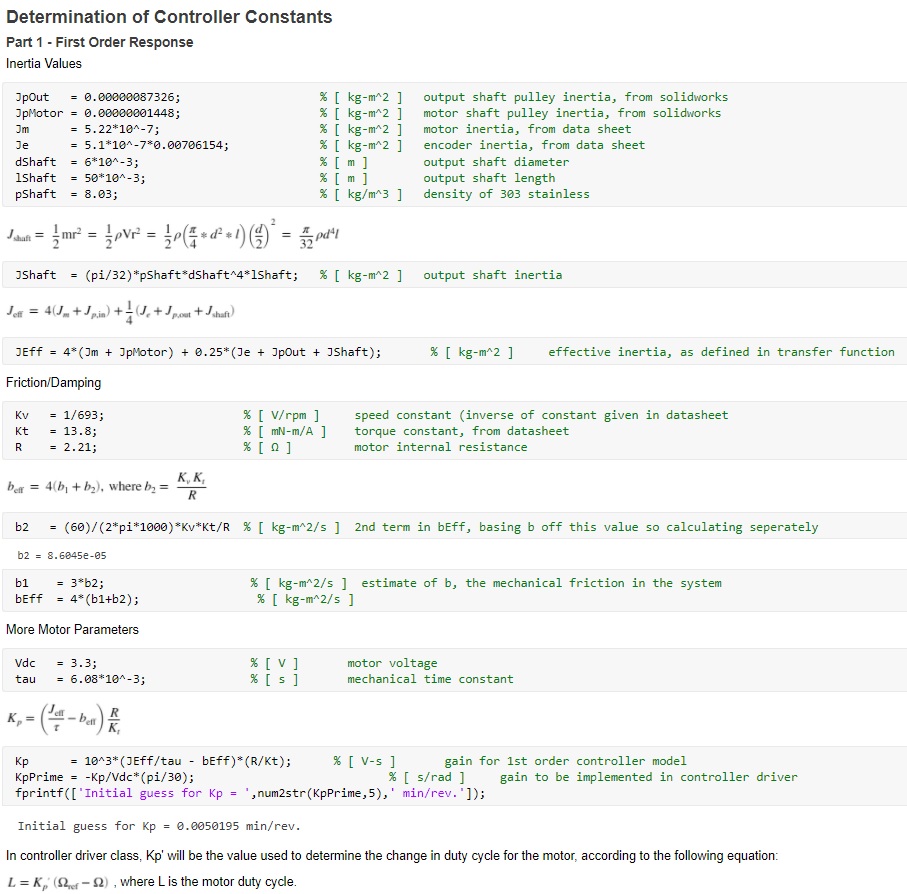
Using equations derived in lecture, an initial guess for K_p was determined (see Figure F.6 below for full derivation). Due to time constraints, K_i was picked solely based on testing.

Figure F.6. Derivation of K_p.

For full documenation of the controller driver class, see closedLoop.closedLoop.

Controller Task

In order to implement a controller, a controller task to run the encoders, motors, and controllers was needed. This file replaced the earlier encoder task, and was in control of 6 different objects (2 encoders, 2 motors, and 2 controllers). Each time a period has elapsed (set from within the main script running all tasks), the workflow of the controller task is the following:

> Get position and speed values from encoders (using methods defined with their respective driver classes)
> Interpolate desired position and speed values from resampled reference data
> Determine the new PWM level for each motor using the controller objects
> Set motors based on controller output

Using this sequence, we can achieve setpoint or reference tracking, depending on the reference data set. See Figure F.7 below for the state transition diagram of the controller task, and see controllerTask.py for full file documentation.

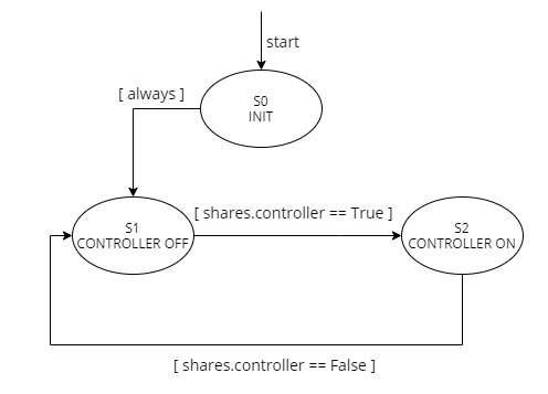
Figure F.7. Controller task state transition diagram developed in week 3.

Note: No changes were made to the controller task finite state machine between weeks 3 and 4, therefore this diagram is only show in week 3.

Week 3 Deliverables

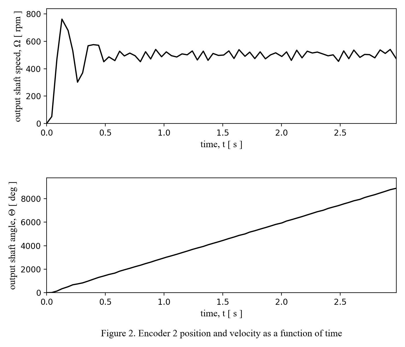
In week 3, our main goal was to determine a K_p value to give us the best system response. Shown below is a progression of tuning plots for the determination of K_p. Note that figure numbers generated directly from Python do not reflect trial numbers, and were only used to differentiate between motors/encoders.

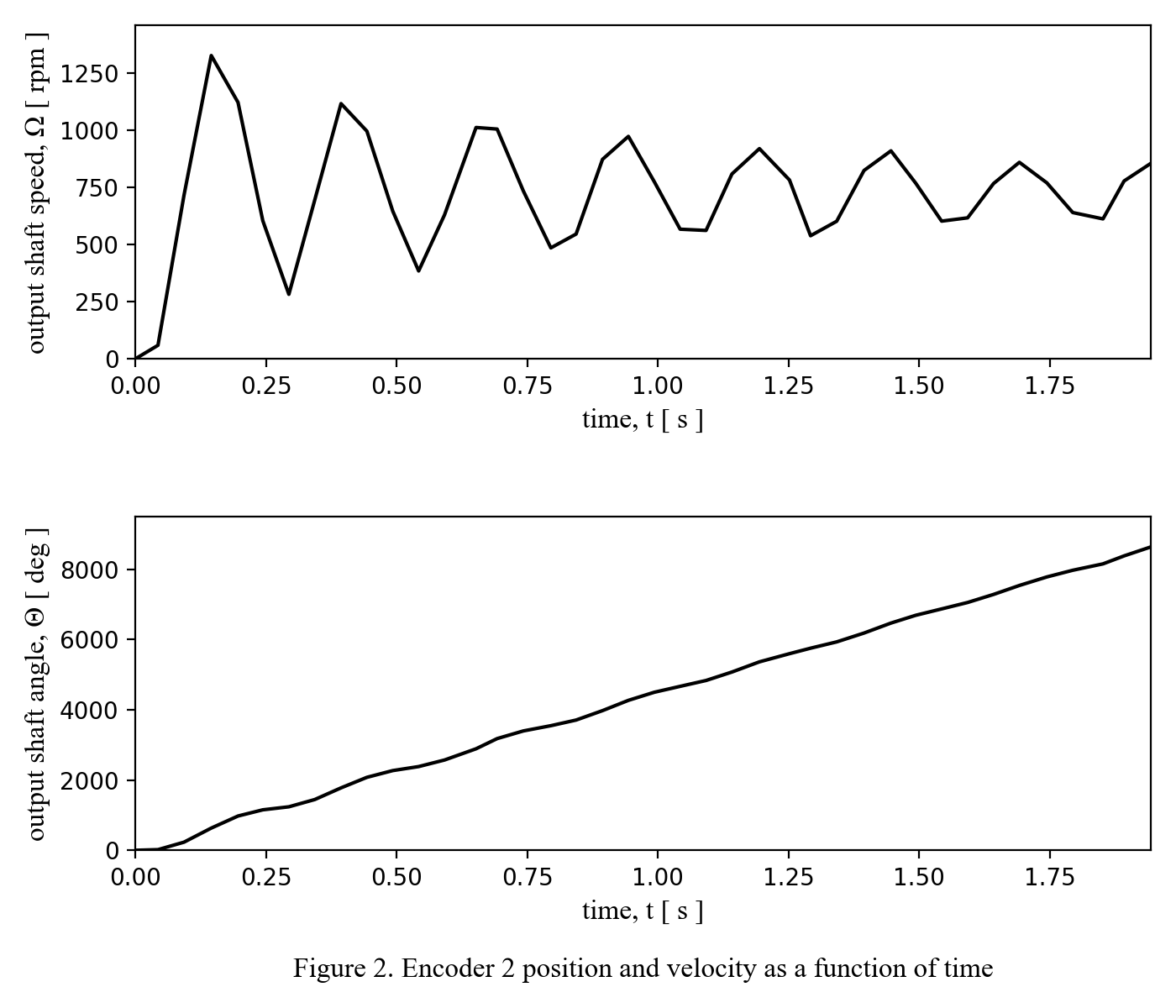
Figure F.8. Initial tuning plot, with K_p set too high.

With K_p set too high, all corrections made to the PWM level were too significant to level out at a given setpoint value. Next, I tried decreasing K_p.

Figure F.9. Decreasing K_p.

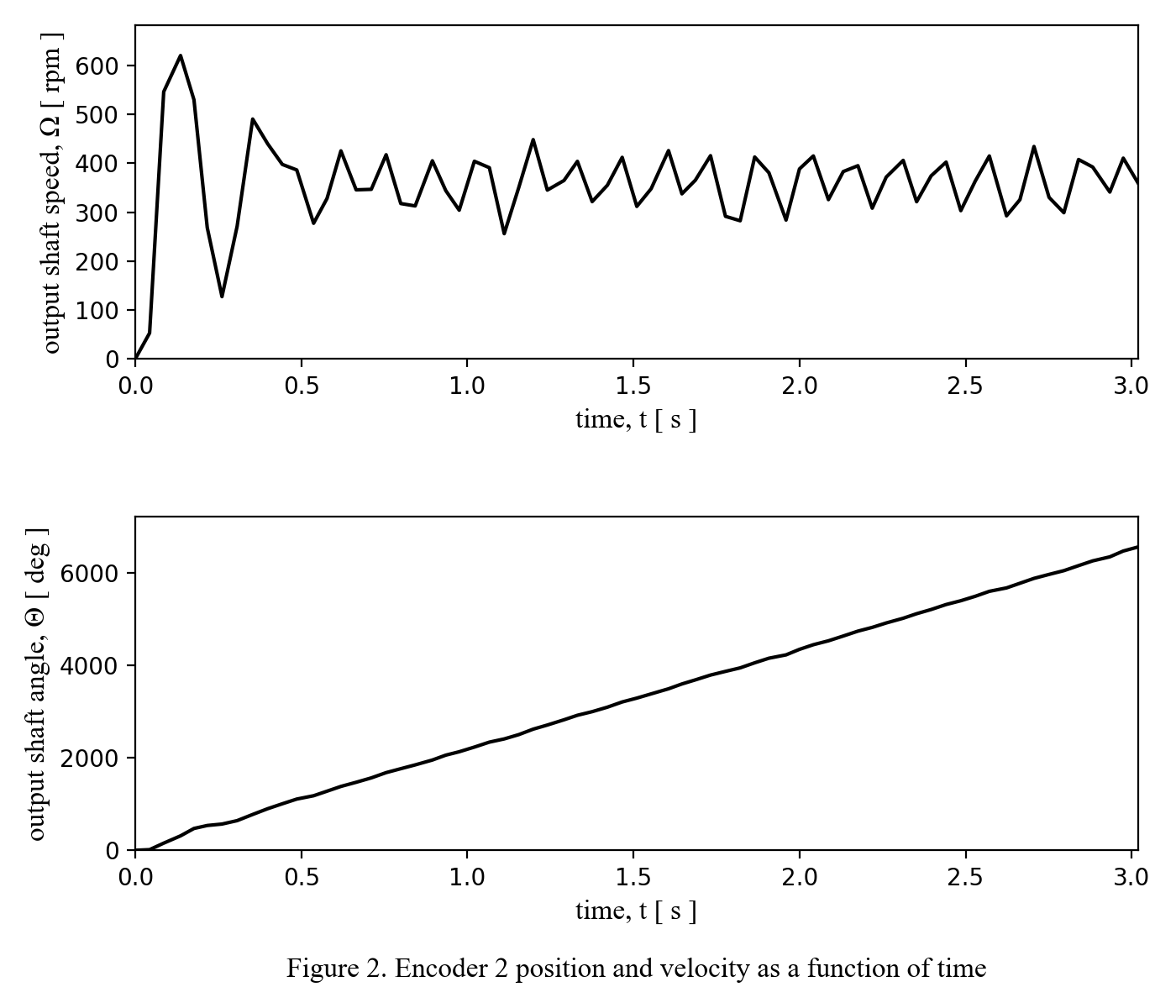
By decreasing K_p, I was able to decrease the fluctuation dramatically from the initial run, but there was still too much oscillation to be functional.

Figure F.10. Decreasing K_p below ideal value.

Again decreasing K_p, this trial resulted in too low of a value for K_p. The final plot below was taken at a value between those used in Figures F.9 and F.10.

Figure F.11. Best trial.

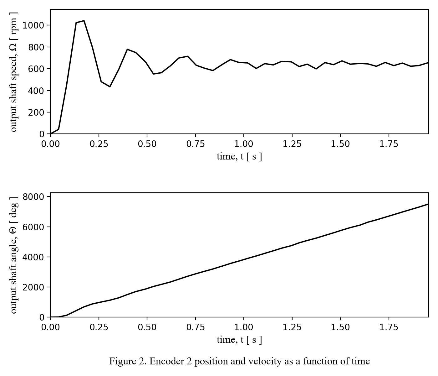
From this tuning, my final value was K_p = 0.05 min/rev. This value would be carried into testing of the final system, but changed slightly with the introduction of PI control.

Click here to advance to Week 4: Switching from Setpoint Tracking to Refrence Tracking.