In the last week of our final projet, no new files/classes were added.

Instead, it was time to modify our code for reference tracking (following a path of predefined, changing speed/position) based on a reference csv. However, given an oversampled data set, we first needed to resamle the data, load it onto the Nucleo, and finally create a method for interpolating from the reference data. A more in-depth description of changes to files previously created, as well as the final refrence tracking plot, can be found below.

Updates to the Front End (PC script)

The first main addition to frontEnd.py was adding a resampling method, sampleCSV, which takes in the sample data, and creates a new csv file, resampled at a given rate. For example, the original data set used for this project was at a rate of 0.001 seconds (1 ms) per data point, whereas the resampled csv had a resolution of .025 s (25 ms). As long as the resampled CSV has a resolution similar to that of the controller period, we will not run into any data issues. The reason for this resampling is mainly for memory concerns on the Nucleo.

In addition to resampling data, the refrence data was plotted together with data collected from encoders to provide a clear visual interpretation of how succesfully the system is working. And lastly, the values used in a given trial for K_p, K_i, and J (our performance metric) were sent through serial to be added as text inside the plot area. To see the final source code for the UI task, see uiTask.py.

Updates to the Controller Task

Some minor changes/additions were made to the controller task, starting with the calculation of J, a performance metric. Each time the controller task updated encoders/motors, the summation portion of J was updated accordingly in the controller task (and in the shared data file shares.py). Then, when the UI sent J to the Front End for displaying on the final plot, the adjusted J value was found by dividing this summation value by the total number of data points taken.

In addition to calculating J, a short method was added for loading data from a CSV file (on the board) into arrays in the controller task file. To see the final source code for the controller task, see controllerTask.py.

Final Task Diagram

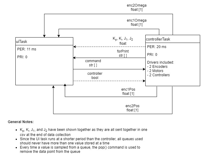
With many variables being shared between files, a task diagram is useful to describe task interactions. See Figure F.12 below for the final system task diagram.

Figure F.12. System task diagram.

Final Results

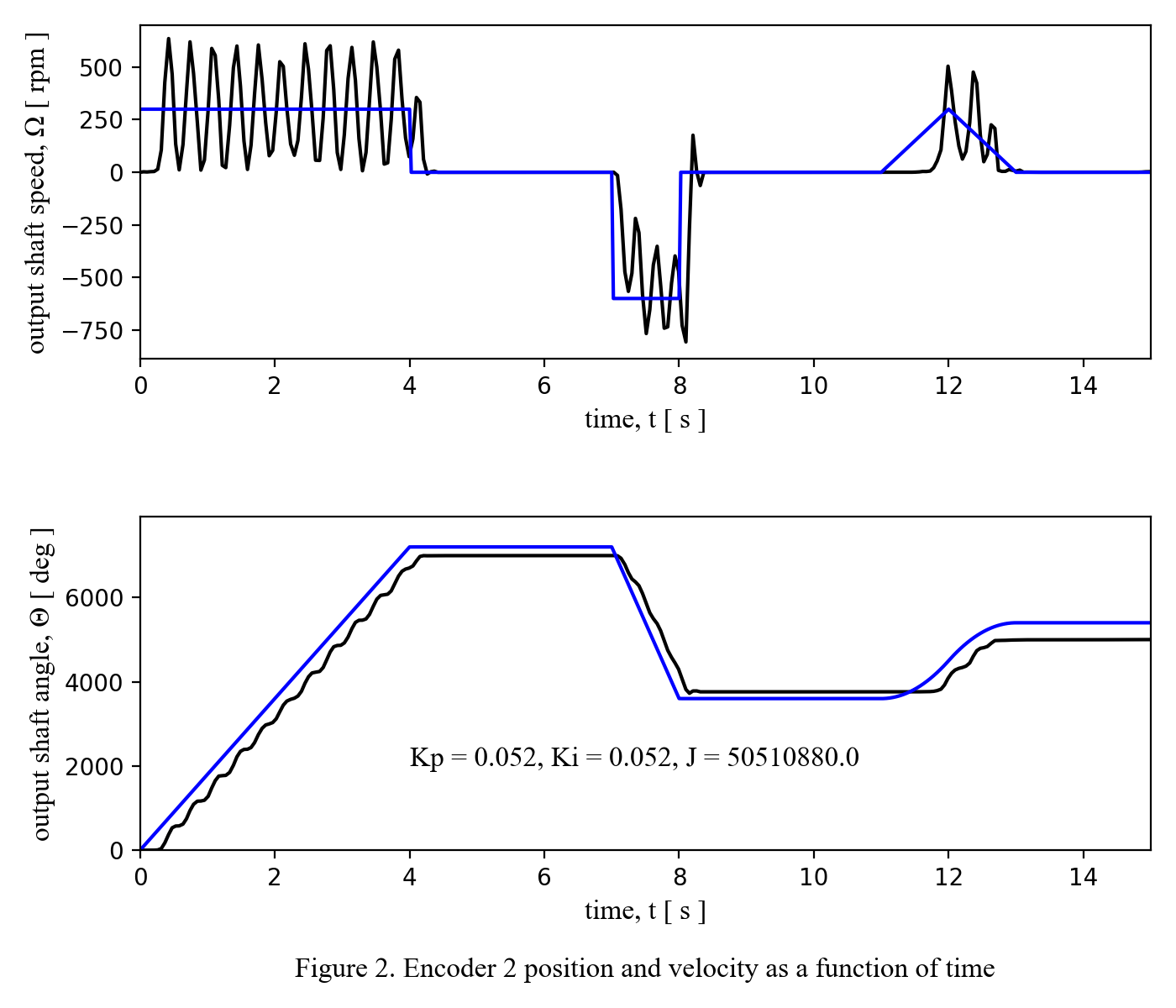
To conclude documentation of this project, the best trial run of the integrated system developed for this project has been shown below. Although J was our agree upon metric for measuring performance, this metric is also not balanced in regards to how errors in position or speed affect the final value, so I based my criteria for "best result" based partially on J, and partially on the visual check of how similar the position data matched the given reference position data.

Figure F.13. Best system plot, with K_p, K_i, and J shown for reference.

Return to Table of Contents.